Detecting Ancient Ink in the Vesuvius Challenge

Vesuvius Challenge 2023 · Gold medal · 8th place

I recently took part in the Vesuvius Challenge Ink Detection competition on Kaggle. Together with yoyobar, we finished in 8th place and earned a gold medal. Our solution combined 3D convolutional networks and SegFormer models, with quite a bit of attention paid to how we sampled the scan layers and stitched the predictions back together.

This was an unusual computer vision problem. Instead of recognizing objects in ordinary photographs, we were trying to detect traces of ink in X-ray scans of ancient papyrus. The scans had a depth dimension, the labeled data came from very few fragments, and the signal we wanted was difficult to distinguish from the material surrounding it.

We have also shared our solution on Kaggle under the title Luck Is All You Need. Here, I will go through the problem, our models, and the inference pipeline in more detail. Hopefully, some of these ideas will be useful to people working on segmentation problems with volumetric data and limited labels.

Problem statement

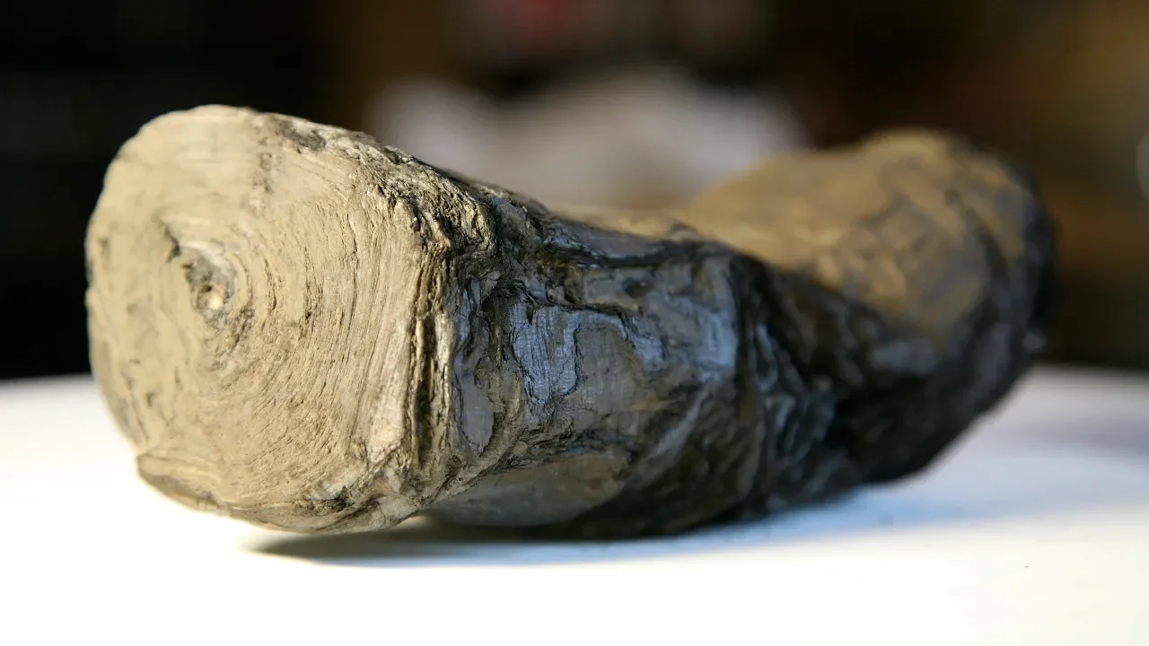
The eruption of Mount Vesuvius in AD 79 buried a library of papyrus scrolls in Herculaneum. The scrolls survived in a carbonized state, but they are so fragile that physically opening them risks destroying them. The broader Vesuvius Challenge aims to recover their contents without unrolling them.

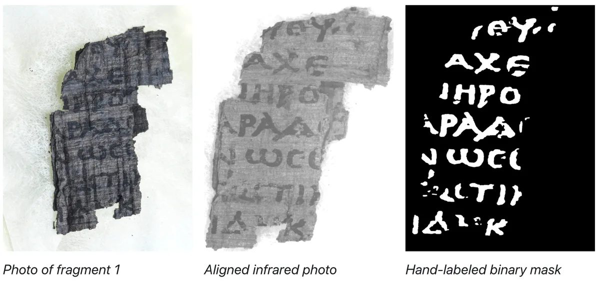
The Kaggle competition addressed one part of that task: detecting ink in 3D X-ray scans of detached papyrus fragments. These fragments provided something a sealed scroll could not readily provide—visible writing that could be used as ground truth. Infrared photographs were aligned with the scans, and hand-labeled masks identified the ink.

This was an ink segmentation task, not a character recognition task. For each surface position, our model had to predict whether ink was present. We were not training a model to translate Greek, recognize individual letters, or virtually unwrap an entire scroll. Competition description

Dataset and evaluation

The training data was organized into three fragments. Each had a stack of scan slices, an ink-label image, and a mask identifying the valid papyrus area. Rather than treating a patch as a conventional RGB image, we could look through a stack of slices near the writing surface and predict a two-dimensional ink mask.

The evaluation used the F0.5 score, which gives precision more weight than recall. A model that marked too much papyrus as ink could therefore suffer even if it recovered many true ink pixels. The final submission contained binary masks encoded with run-length encoding. This made thresholding an important part of the solution, rather than just a formatting step after training. Evaluation details

Local validation

Having a large number of patches did not mean we had a large number of independent examples. Patches cut from the same fragment share its texture, scan characteristics and local structure. A random patch split could give an overly optimistic impression of how well a model would perform on another fragment.

We tried two cross-validation schemes. The first held out each of the three fragments in turn. The second split fragment 2 into a top and bottom half, giving four regions: fragment 1, fragment 2a, fragment 2b and fragment 3. Different members of the final ensemble used different schemes; the large 3D SE-ResNet model used a single validation region, fragment 2a.

The four-region split gave us another view of the data, but it did not create another independent fragment. That distinction is worth keeping in mind when comparing validation scores.

Preprocessing and augmentation

We capped normalized pixel intensities at 0.78. We also trained with three spatial scales: the original resolution, 0.75× and 0.5×. This let the models encounter the same writing and papyrus structure at different apparent sizes.

The depth dimension gave us additional ways to augment the data. We used compression along the z-axis, small 3D rotations, channel dropout, and ordinary spatial rotations and flips. The depth compression varied by approximately ±20%, and the 3D rotation by approximately ±5°.

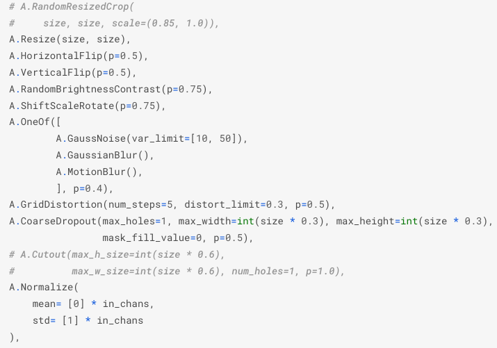
The Albumentations pipeline also included brightness and contrast changes, noise or blur, shift-scale-rotate, grid distortion and coarse dropout. These transformations varied the appearance of the patches without requiring additional labeled fragments. As usual for segmentation, spatial transformations had to be applied consistently to both the input and its label.

Models

Our final solution consisted of five model configurations built around three encoder families: 3D SE-ResNet-101, 3D ResNet-34 and SegFormer-B3. The important difference was not just the backbone name. These models processed the depth information in different ways.

3D SE-ResNet-101

The 3D SE-ResNet model used a modified encoder with squeeze-and-excitation layers and dilated convolutions. We used BasicBlock rather than Bottleneck blocks and trained the model from scratch, without pretrained weights.

Training proceeded in two stages. We started with 96-pixel patches, which were easier to train, then continued with larger patches of 192 and 256 pixels. The final ensemble used the 256-pixel configuration.

For this model, we sampled a 20-slice depth window from the region between slices 15 and 40. During inference, we moved that window through the depth range in steps of five slices and averaged the predictions. This was our “channel TTA”: instead of committing to a single depth window, we combined predictions from multiple nearby windows.

The training loss combined binary cross-entropy and Dice loss. Areas outside the valid papyrus mask were excluded.

SegFormer-B3

We also used an ImageNet-pretrained SegFormer-B3 encoder with three-channel inputs. Here the channels were scan slices, not red, green and blue. The question was how to use more depth information while retaining a model that accepted three slices at a time.

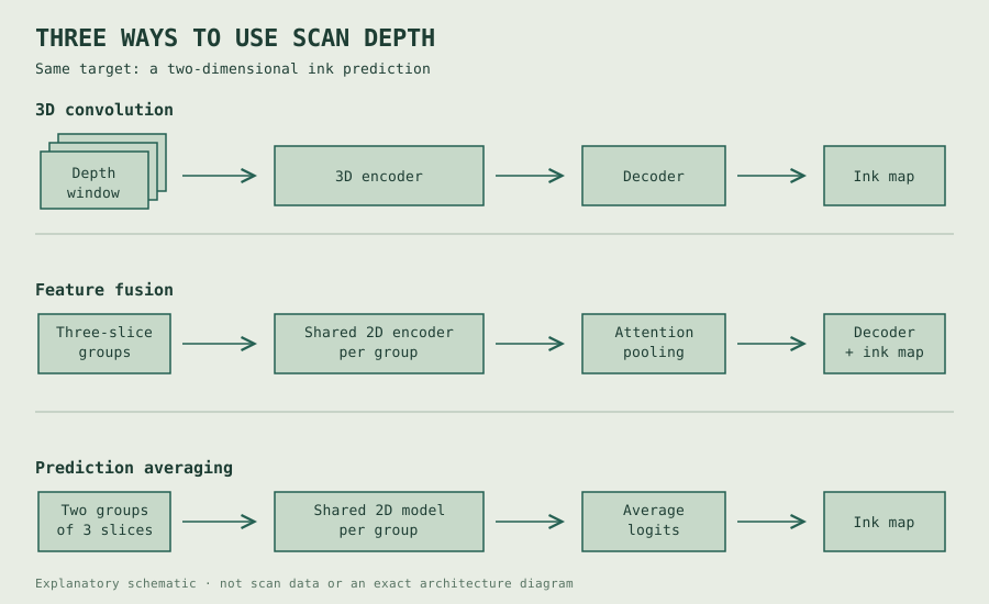
We tried two approaches. In the first, we processed groups of three slices and combined their feature maps with attention pooling. The idea was to let the model learn how to combine evidence from different depths before decoding the segmentation. hengck23's discussion of attention pooling was a useful reference.

The second approach was simpler: take six slices, divide them into two groups of three, pass both through the same model, and average the output logits. Rather than learning an additional feature-fusion mechanism, this combined the predictions from the two groups directly.

Both configurations used 224-pixel inputs and binary cross-entropy loss, again excluding areas outside the papyrus mask.

3D ResNet-34

The remaining two configurations used a 3D ResNet-34 encoder, with input sizes of 224 and 192 pixels. They used 18-slice inputs and a combination of binary cross-entropy and Dice loss.

These provided another way of extracting features from the scan volume, alongside the larger SE-ResNet and the grouped-slice SegFormer models. The final ensemble therefore varied the encoder, spatial resolution, depth treatment and validation scheme, rather than only repeating one model with different random seeds.

Inference and stitching

The fragments were much larger than the model inputs, so we ran inference on overlapping patches and reconstructed a full prediction map. We used FP16 inference, 90-degree rotation test-time augmentation, and channel TTA for the SE-ResNet model. Predictions outside the papyrus mask were ignored.

One important detail was to discard the outer part of each predicted patch and retain only its center. Pixels near the boundary of a patch have less surrounding context, so their predictions can differ from those obtained when the same pixels appear nearer the center of another patch. Overlapping center crops let us cover the fragment without depending on those edge predictions.

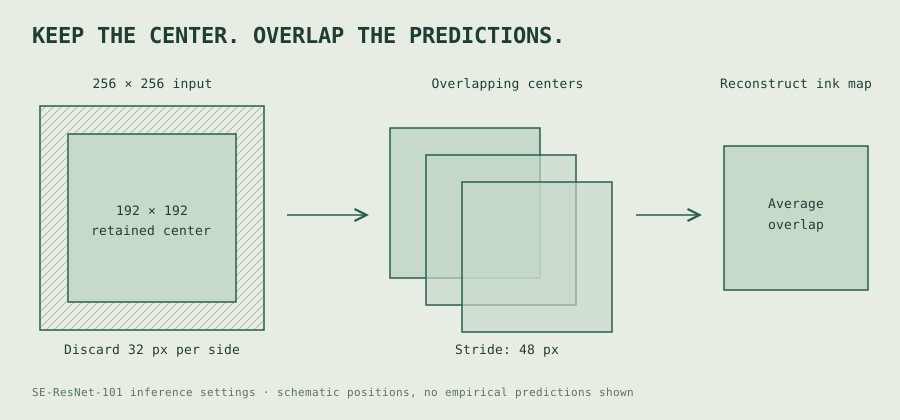
The crop sizes and strides differed by model:

Model configuration	Input size	Retained output size	Inference stride	Validation scheme
3D SE-ResNet-101	256	192	48	Single fold, fragment 2a
SegFormer-B3 with attention pooling	224	160	80	Four folds
SegFormer-B3 with averaged logits	224	176	88	Three folds
3D ResNet-34	224	192	96	Four folds
3D ResNet-34	192	160	80	Three folds

These are inference settings; they should not be confused with the patch-sampling stride used during training. We also list them in our Kaggle solution write-up.

Final ensemble and thresholding

We formed our team in the last week of the competition. Most of our experiments had been done independently, which is why the released repository retains separate felix_work and yoyobar_work directories. The final inference pipeline brought the models together through weighted averaging.

We selected two final submissions. One applied a fixed threshold of 0.55. The other used a percentile-based strategy, selecting approximately the highest-scoring 3% of pixels.

These choices make different assumptions. A fixed threshold assumes that the prediction scores remain sufficiently calibrated on new data. A percentile threshold depends more on the ranking of pixels, but imposes an assumption about how much ink should be present. Neither assumption is guaranteed to hold for an unseen fragment.

Both submissions scored about 0.79 on the public leaderboard. On the private leaderboard, the fixed-threshold submission scored about 0.65, while the percentile-based submission scored about 0.63. The fixed threshold performed better, with final scores of 0.792859 public and 0.655514 private. Kaggle write-up, reproduction instructions

Methods that did not work

Not every addition improved the solution. We tried adding a Convolutional Block Attention Module to the decoder of the 3D ResNet, but the cross-validation score dropped. Using the infrared image as an additional segmentation head did not improve validation either. Mixup and label-noise augmentation were also among the methods that did not make it into the final solution.

These results do not mean that the methods are ineffective in general. They mean that, in the configurations we tested, they did not improve our validation results enough to use them. With very little independent labeled data, additional architectural complexity is not automatically an advantage.

Lessons

The depth dimension deserves its own experiments

Depth was not simply another set of channels to feed into a larger network. Our solution used 3D convolutions, grouped-slice feature pooling, grouped-slice logit averaging, and sliding depth windows at inference. These are different assumptions about how information across slices should be combined.

For a similar problem, I would make the depth representation an explicit part of the experiment plan, alongside the backbone and loss. A model can only use the information that its input representation makes available.

Validation is limited by the number of independent fragments

This reminded me of the validation problem in my Nature Conservancy fisheries competition. There, many images came from the same boats. Here, many patches came from the same papyrus fragments. In both cases, counting training examples can hide how little independent variation the dataset actually contains.

Fragment-level validation is more informative than a random patch split, but three fragments still give a limited view of generalization. The public-to-private score drop is also a reason not to treat a strong public leaderboard score as a complete assessment of the model.

Inference is part of the model

The final output depended on more than the trained weights. Depth-window selection, rotations, overlap, center cropping, ensemble weights and thresholding all affected the binary mask we submitted. These settings deserve to be recorded and tested just as carefully as the architecture.

The threshold comparison is a concrete example: two submissions could look similar on the public leaderboard and still differ on the private data. A useful validation pipeline needs to evaluate the complete inference procedure, not just the training loss or isolated patch predictions.

Code and acknowledgements

We have open-sourced the complete solution and reproduction instructions, including data preparation, model training and inference. My experiments ran on a single RTX 3090 with 64 GB of RAM; yoyobar used a single RTX 4090 with 80 GB of RAM.

Thanks to yoyobar, the competition organizers, and everyone who shared ideas and notebooks during the competition. In particular, hengck23's explanation of attention pooling was helpful for the SegFormer approach.

The competition was a chance to apply familiar deep-learning tools to a very unfamiliar dataset. Finishing in 8th place was rewarding, but so was working on a problem where better segmentation could contribute to recovering writing that had been inaccessible for centuries.